반응형
Average ROC for repeated 10-fold cross validation with probability estimates
I am planning to use repeated (10 times) stratified 10-fold cross validation on about 10,000 cases using machine learning algorithm. Each time the repetition will be done with different random ...
stats.stackexchange.com
여기 Stackexchange 사이트에 해당 답변이 아주 잘 구현되어 있다.
그런데 Python으로 그리는 Figure는 ppt에서 수정을 할 수가 없다 ㅠㅠ
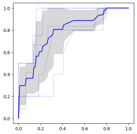
그래서 일단 Python으로 5-fold cross validation의 평균 ROC를 구해보고,
그리고 같은 코드를 R로도 작성해본다.
1. Python (5-fold cross validation)
## Library import
import matplotlib.pyplot as plt
import numpy as np
from sklearn.metrics import roc_curve
import pandas as pd
## Data load
tmp = [[0.165,0,1], [0.445,1,1], [0.675,1,1], [0.16,0,1], [0.425,0,1], [0.375,0,1], [0.085,0,1], [0.055,0,1], [0.125,0,1], [0.475,0,1], [0.14,0,1], [0.005,0,1], [0.135,0,1], [0.05,0,1], [0.205,0,1],
[0.545,0,1], [0.38,0,1], [0.625,0,1], [0.185,0,1], [0.3,0,1], [0.09,0,1], [0.155,0,1], [0.095,0,1], [0.065,0,1], [0.05,0,1], [0.465,0,1], [0.42,0,1], [0.085,0,2], [0.68,1,2], [0.265,1,2],
[0.39,1,2], [0.08,0,2], [0.12,0,2], [0.22,0,2], [0.055,0,2], [0.045,0,2], [0.375,0,2], [0.19,0,2], [0.58,0,2], [0.415,0,2], [0.205,0,2], [0.24,0,2], [0.12,0,2], [0.16,0,2], [0.145,0,2], [0.045,0,2],
[0.095,0,2], [0.105,0,2], [0.115,0,2], [0.135,0,2], [0.585,0,2], [0.11,0,2], [0.385,0,2], [0.62,1,2], [0.1,1,3], [0.185,1,3], [0.46,0,3], [0.24,1,3], [0.615,1,3], [0.165,1,3], [0.565,0,3],
[0.225,0,3], [0.1,0,3], [0.485,0,3], [0.045,0,3], [0.165,0,3], [0.125,0,3], [0.01,0,3], [0.155,0,3], [0.095,0,3], [0.115,0,3], [0.395,0,3], [0.06,0,3], [0.105,0,3], [0.04,0,3], [0.37,0,3],
[0.165,0,3], [0.025,0,3], [0.29,0,3], [0.23,0,3], [0.27,0,3], [0.31,1,4], [0.18,1,4], [0.045,1,4], [0.135,1,4], [0.025,1,4], [0.135,1,4], [0.12,1,4], [0.115,1,4], [0.13,1,4], [0.385,1,4],
[0.32,1,4], [0.045,0,4], [0.045,0,4], [0.125,0,4], [0.005,0,4], [0.01,0,4], [0.07,0,4], [0.065,0,4], [0.19,1,4], [0.05,0,4], [0.17,0,4], [0.07,0,4], [0.005,0,4], [0.335,0,4], [0.125,0,4],
[0.085,0,4], [0.055,0,4], [0.09,1,5], [0.4,1,5], [0.35,1,5], [0.595,1,5], [0.36,1,5], [0.08,0,5], [0.065,0,5], [0.35,0,5], [0.335,0,5], [0.145,0,5], [0.125,0,5], [0.5,0,5], [0.25,0,5], [0.57,0,5],
[0.175,0,5], [0.275,0,5], [0.145,0,5], [0.36,0,5], [0.15,0,5], [0.055,0,5], [0.365,0,5], [0.055,0,5], [0.055,0,5], [0.495,0,5], [0.345,0,5], [0.565,0,5], [0.29,0,5]]
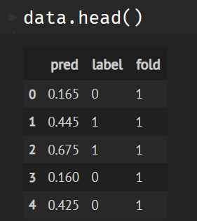
data = pd.DataFrame(tmp, columns=['pred','label', 'fold'])
그러면 data는 다음과 같이 생성된다.
## 시각화
import numpy as np
import matplotlib.pyplot as plt
from sklearn.metrics import roc_curve

tprs = []

# 기본 False Positive Rate (거짓 양성 비율) 범위 설정
base_fpr = np.linspace(0, 1, 101)

plt.figure(figsize=(5, 5))
plt.axes().set_aspect('equal', 'datalim')

for fold in range(1, 6):
    foldRes = data.loc[data['fold'] == fold]
    fpr, tpr, _ = roc_curve(foldRes['label'], foldRes['pred'])

    plt.plot(fpr, tpr, 'b', alpha=0.15)
    # TPR 값을 기본 FPR에 대해 보간
    tpr = np.interp(base_fpr, fpr, tpr)
    tpr[0] = 0.0
    tprs.append(tpr)

tprs = np.array(tprs)
mean_tprs = tprs.mean(axis=0)
std = tprs.std(axis=0)

# 상한과 하한을 계산하여 신뢰구간 생성
tprs_upper = np.minimum(mean_tprs + std, 1)
tprs_lower = mean_tprs - std

# 평균 ROC curve와 신뢰구간을 시각화
plt.plot(base_fpr, mean_tprs, 'b')
plt.fill_between(base_fpr, tprs_lower, tprs_upper, color='grey', alpha=0.3)
2. R (5-fold cross validation)
## Data load
tmp = rbind(c(0.165,0,1), c(0.445,1,1), c(0.675,1,1), c(0.16,0,1), c(0.425,0,1), c(0.375,0,1), c(0.085,0,1), c(0.055,0,1), c(0.125,0,1), c(0.475,0,1), c(0.14,0,1), c(0.005,0,1), c(0.135,0,1), c(0.05,0,1), c(0.205,0,1),
    c(0.545,0,1), c(0.38,0,1), c(0.625,0,1), c(0.185,0,1), c(0.3,0,1), c(0.09,0,1), c(0.155,0,1), c(0.095,0,1), c(0.065,0,1), c(0.05,0,1), c(0.465,0,1), c(0.42,0,1), c(0.085,0,2), c(0.68,1,2), c(0.265,1,2),
    c(0.39,1,2), c(0.08,0,2), c(0.12,0,2), c(0.22,0,2), c(0.055,0,2), c(0.045,0,2), c(0.375,0,2), c(0.19,0,2), c(0.58,0,2), c(0.415,0,2), c(0.205,0,2), c(0.24,0,2), c(0.12,0,2), c(0.16,0,2), c(0.145,0,2), c(0.045,0,2),
    c(0.095,0,2), c(0.105,0,2), c(0.115,0,2), c(0.135,0,2), c(0.585,0,2), c(0.11,0,2), c(0.385,0,2), c(0.62,1,2), c(0.1,1,3), c(0.185,1,3), c(0.46,0,3), c(0.24,1,3), c(0.615,1,3), c(0.165,1,3), c(0.565,0,3),
    c(0.225,0,3), c(0.1,0,3), c(0.485,0,3), c(0.045,0,3), c(0.165,0,3), c(0.125,0,3), c(0.01,0,3), c(0.155,0,3), c(0.095,0,3), c(0.115,0,3), c(0.395,0,3), c(0.06,0,3), c(0.105,0,3), c(0.04,0,3), c(0.37,0,3),
    c(0.165,0,3), c(0.025,0,3), c(0.29,0,3), c(0.23,0,3), c(0.27,0,3), c(0.31,1,4), c(0.18,1,4), c(0.045,1,4), c(0.135,1,4), c(0.025,1,4), c(0.135,1,4), c(0.12,1,4), c(0.115,1,4), c(0.13,1,4), c(0.385,1,4),
    c(0.32,1,4), c(0.045,0,4), c(0.045,0,4), c(0.125,0,4), c(0.005,0,4), c(0.01,0,4), c(0.07,0,4), c(0.065,0,4), c(0.19,1,4), c(0.05,0,4), c(0.17,0,4), c(0.07,0,4), c(0.005,0,4), c(0.335,0,4), c(0.125,0,4),
    c(0.085,0,4), c(0.055,0,4), c(0.09,1,5), c(0.4,1,5), c(0.35,1,5), c(0.595,1,5), c(0.36,1,5), c(0.08,0,5), c(0.065,0,5), c(0.35,0,5), c(0.335,0,5), c(0.145,0,5), c(0.125,0,5), c(0.5,0,5), c(0.25,0,5), c(0.57,0,5),
    c(0.175,0,5), c(0.275,0,5), c(0.145,0,5), c(0.36,0,5), c(0.15,0,5), c(0.055,0,5), c(0.365,0,5), c(0.055,0,5), c(0.055,0,5), c(0.495,0,5), c(0.345,0,5), c(0.565,0,5), c(0.29,0,5))

data = data.frame(tmp)
colnames(data) <- c("pred", "label", "fold")
## 5-fold에서 tpr 구하여 리스트에 저장
# by, lapply를 써서 조금 이해하기 어려울 수 있겠지만, 그냥 fold 별로 roc를 구하고 cbind로 묶음
base_fpr <- seq(0, 1, by = 0.01)
roc_obj_list = by(data, INDICES=data$fold, function(x) pROC::roc(x$label ~ x$pred))
tpr_interp <- lapply(roc_obj_list, function(roc_obj) approx(1 - roc_obj$specificities, roc_obj$sensitivities, xout = base_fpr)$y)
mean_tpr = do.call(cbind, tpr_interp)
## 보간법을 활용하여 base_fpr에 따른 평균 tpr 및 CI 구하기
mean_tprs <- rowMeans(mean_tpr, na.rm = TRUE)
std_tprs <- apply(mean_tpr, 1, sd, na.rm = TRUE)

tprs_upper <- pmin(mean_tprs + std_tprs, 1)
tprs_lower <- mean_tprs - std_tprs

final_df <- data.frame(
  FPR = base_fpr,
  TPR = mean_tprs,
  Upper = tprs_upper,
  Lower = tprs_lower
)
final_df <- rbind(rep(0, 4), final_df)
#마지막에 0을 추가해주는 이유는 pROC의 roc가 원점 (0,0)을 통과하지 않는 경우가 있기 때문..
마지막 최종 시각화
gg <- ggplot(final_df, aes(x = FPR)) +
  geom_line(aes(y = TPR), color = "blue") +
  geom_ribbon(aes(ymin = Lower, ymax = Upper), alpha = 0.3) +
  xlim(0, 1) + ylim(0, 1) + coord_fixed() + theme_bw()
print(gg)
제가 논문 figure 시각화 할 때 theme_bw()를 좋아하는데, 그건 취향에 맞춰서..
'Major Study. > Bioinformatics' 카테고리의 다른 글
| Radiology reports의 Causal relationship (0) | 2023.12.14 |
|---|---|
| DINO Contrastive Learning in Medical Imaging (2) | 2023.11.17 |
| Histopathology를 다루기 위한 MIL (1) | 2023.02.26 |
| Single Cell Analysis Best Practice 정리해보기 (1) | 2023.02.06 |
| GTEx에서 Pathology image 분석하기 (0) | 2022.10.13 |